
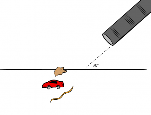
A snowmobile moving at constant speed drags a load, as shown in the picture. The coefficient of kinetic friction between the load and the ice is \(\mu\).
(a) Calculate the tension in the rope that connects the load to the snowmobile, in terms of m, g, \(\theta\) and \(\mu\).
(b) Describe what would happen if \(\theta\) is close to zero, and what would happen if \(\theta\) is close to 90 degrees.
a) The tension is the only force that has components along both the \({x-}\) and \({y-}\)axes. Draw a free body diagram and break the force vectors into components to find the tension force.
b) Evaluate each case using the equation obtained for the tension force from part (a).
a) Newton’s Second Law in the \({x-}\)direction, remembering that the object is moving at constant speed, can be written as:
\begin{equation*}
-f_r+T\cos(\theta)=0,
\end{equation*}
where \(f_r = \mu N\). Newton’s Second Law in the \({y-}\)direction is:
\begin{equation*}
N + T \sin \theta – mg = 0.
\end{equation*}
Solving for \(N\) substituting it into the first equation, and then solving for \(T\) yields:
\begin{equation*}
T=\frac{\mu mg}{\mu \sin(\theta)+\cos(\theta)}.
\end{equation*}
b) If \(\theta \to 0 \), then:
\begin{equation*}
T=\mu mg,
\end{equation*}
which means that \(T\) must be horizontal.
If \(\theta \to 90^\circ \), then there will be no forces in the \({x-}\)direction. Numerically, we get:
\begin{equation}
T=\frac{\mu m g}{\mu +0}= m g.
\end{equation}
For a more detailed explanation of any of these steps, click on “Detailed Solution”.
1. General Strategy for (a)
a) They’ve asked us to find the tension in the rope. To solve this problem, we’ll start by making a free-body diagram identifying all the forces exerted on the load. Then, we’ll use Newton’s second law in the X and Y axis to solve for the tension \(T\).
2. Identify the forces and make a free body diagram
To make the the free-body diagram, we first identify the forces (we will be using a coordinate system with Y pointing upwards and X pointing in the direction of motion). The forces are:
- The weight \(W=mg\) directed in the negative Y axis. Here \(m\) is the mass of the load and \(g\) the gravitational acceleration on Earth.
- The contact force with the floor \(N\), which is normal to the surface and thus is directed along the positive Y axis.
- The kinetic friction \(f_r\) directed along the negative X axis (opposing the movement between the surfaces). Its magnitude will be the kinetic coefficient of friction \(\mu\) multiplied by the contact force \(N\), namely \(fr=\mu N\).
- The tension exerted by the rope \(T\) at an angle \(\theta\) from the X axis. We can thus decompose the force by components.
Hence, the free-body diagram can be shown in figure 1.

Figure 1: Free-body diagram of the load with the following forces: the weight \(\vec{W}\), the contact force with the ground \(\vec{N}\), the tension \(\vec{T}\), and the friction \(\vec{f}_r\). The angle that the tension makes with the horizontal axis and its decomposition along the X and Y axis are also shown. The coordinate system is chosen so that X is along the direction of movement and Y points upwards.
3. Newton’s Second Law in X
We can then write Newton’s second law for the X axis as
\begin{equation}
\label{newtonx1}
-f_r\,\hat{\textbf{i}}+T_x\,\hat{\textbf{i}}=ma_x\,\hat{\textbf{i}},
\end{equation}
where \(a_x\) is the acceleration along the X axis and \(T_x\) the tension in X. From the free-body diagram, we see that the component along the X axis will be \(T\cos(\theta)\).
Hence, the previous equation becomes
\begin{equation}
\label{newtonx}
-f_r\,\hat{\textbf{i}}+T\cos(\theta)\,\hat{\textbf{i}}=ma_x\,\hat{\textbf{i}}.
\end{equation}
Because the snowmobile moves with constant speed, so does the load, meaning that the acceleration is zero \(a_x=0\). Thus, equation \eqref{newtonx} can be written as
\begin{equation}
-f_r\,\hat{\textbf{i}}+T\cos(\theta)\,\hat{\textbf{i}}=0\,\hat{\textbf{i}},
\end{equation}
or dropping the vector notation and focusing on the magnitude of each vector, we get
\begin{equation}
-f_r+T\cos(\theta)=0.
\end{equation}
Additionally, we can use that \(fr=\mu N\) to write the equation above as
\begin{equation}
\label{newtonx2}
-(\mu N)+T\cos(\theta)=0.
\end{equation}
4. Newton’s Second Law in Y
Now, we write Newton’s second law for the Y axis:
\begin{equation}
-mg\,\hat{\textbf{j}}+N\,\hat{\textbf{j}}+T_y\,\hat{\textbf{j}}=ma_y\,\hat{\textbf{j}},
\end{equation}
where \(a_y\) is the acceleration along the Y axis and \(T_y\) the Y component of the tension. From the force diagram, we see that this component equals \(T\sin(\theta) \).
\begin{equation}
-mg\,\hat{\textbf{j}}+N\,\hat{\textbf{j}}+T\sin(\theta)\,\hat{\textbf{j}}=ma_y\,\hat{\textbf{j}}.
\end{equation}
Since the load does not move vertically along the Y axis, its acceleration along this direction is zero \(a_y=0\). Thus, we can write Newton’s second law for the Y axis as
\begin{equation}
-mg\,\hat{\textbf{j}}+N\,\hat{\textbf{j}}+T\sin(\theta)\,\hat{\textbf{j}}=0\,\hat{\textbf{j}},
\end{equation}
or dropping the vector notation and focusing on the magnitudes
\begin{equation}
-mg+N+T\sin(\theta)=0.
\end{equation}
5. Manipulate equations
We can solve for \(N\) in the equation above. Explicitly,
\begin{equation}
\label{normal}
N=mg-T\sin(\theta).
\end{equation}
Using this result for \(N\) in equation \eqref{newtonx2}, we obtain
\begin{equation}
-\mu(mg-T\sin(\theta))+T\cos(\theta)=0.
\end{equation}
Expanding the term in parenthesis in the expression above, we obtain
\begin{equation}
\label{casi}
-\mu mg+ \mu T\sin(\theta)+T\cos(\theta)=0.
\end{equation}
From equation \eqref{casi} we can solve for the tension \(T\) in terms of the required variables. Let’s start by factorizing \(T\) in the last two terms of equation \eqref{casi} to get
\begin{equation}
-\mu mg +T(\mu \sin(\theta)+\cos(\theta))=0.
\end{equation}
Now, let’s add up \(\mu m g\) on both sides of the equation to get
\begin{equation}
T(\mu \sin(\theta)+\cos(\theta))=\mu mg.
\end{equation}
Dividing both sides by the term \(\sin(\theta)+\cos(\theta)\), we finally get
\begin{equation}
\label{result}
T=\frac{\mu mg}{\mu \sin(\theta)+\cos(\theta)}.
\end{equation}
6. General Strategy for (b)
b) For the last part of the problem, we need to discuss what would happen if \(\theta\) is close to zero and 90 degrees. Hence, we need to adapt the equation for \(T\) for this case.
7. Adapt previous equations to the new situation
As the angle \(\theta\) approaches zero, the expression for \(T\) becomes
\begin{equation}
T=\frac{\mu mg}{\mu \sin(0^{\circ})+\cos(0^{\circ})},
\end{equation}
which is
\begin{equation}
\label{t0}
T=\frac{\mu m g}{0+1}=\mu mg.
\end{equation}
Notice as \(T\) approaches zero, the direction of the tension will be totally horizontal. Thus, in the Y axis there will only be two forces, the contact force \(N\) and the weight \(mg\). From the equilibrium condition (the fact that there is no acceleration), these two forces must be equal, and so \(N=mg\). In the X axis there will be only two forces too, the friction \(f_r\) and the tension \(T\). The result of equation \eqref{t0} reflects this fact because from \(f_r=\mu N\) together with the results for the Y axis, we get \(f_r=\mu mg\).
As the angle increases, the value of \(T\) decreases and reaches a minimum value at \(\theta=45\) degrees. For an angle close to \(\theta=90\) degrees, the tension will be mostly along the Y axis. Using the result of equation \eqref{result}, we get
\begin{equation}
T=\frac{\mu mg}{\mu \sin(90^{\circ})+\cos(90^{\circ})},
\end{equation}
which simplifies to
\begin{equation}
T=\frac{\mu m g}{\mu +0}= m g.
\end{equation}
As the angle approaches 90 degrees, the tension is again maximum; however, we must be extra careful with this case because as the tension approaches 90 degrees, the friction with the floor decreases, becoming zero when \(\theta=90^{\circ}\), which means there will be no forces exerted on the load along the X axis! And this will contradict the fact that the load is moving at constant speed on a surface with friction.

Leave A Comment