
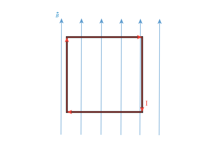
A square wire loop of side 65 cm, carrying a clockwise current of 4.3 A, is oriented parallel to a uniform magnetic field of 3.5 T.
a) What is the force on each side of the loop?
b) Calculate the net force and torque that the magnetic field exerts on the loop.
a) Use the definition of the magnetic force in terms of the current and the length. Then, by defining each vector length, you can find the magnetic force for each cable.
b) The torque can be found with the magnetic moment and the magnetic field.
a) The magnetic force is:
\begin{equation*}
\vec{F}=I\vec{L}\times\vec{B}.
\end{equation*}
Since \(\vec{B} = B \ \hat{\textbf{j}} \), and with \(\vec{L}_1 = – L \ \hat{\textbf{j}} \), then:
\begin{equation*}
\vec{F}_1=\vec{0}.
\end{equation*}
For \(\vec{L}_2 = – L \ \hat{\textbf{i}} \), then:
\begin{equation*}
\vec{F}_2= -ILB \ \hat{\textbf{k}} \approx -9.78 \, \text{N} \ \hat{\textbf{k}}.
\end{equation*}
For \(\vec{L}_3 = L \ \hat{\textbf{j}} \), then:
\begin{equation*}
\vec{F}_3= 0.
\end{equation*}
For \(\vec{L}_4 = L \ \hat{\textbf{i}} \), then:
\begin{equation*}
\vec{F}_4= ILB \ \hat{\textbf{k}} \approx 9.78 \, \text{N} \ \hat{\textbf{k}}.
\end{equation*}
b) The magnetic moment of the wire is:
\begin{equation*}
\vec{\mu}=IA\,\hat{\textbf{n}},
\end{equation*}
where in this case \( \vec{\mu} = – IL^2 \ \hat{\textbf{k}} \). Then, the torque is:
\begin{equation*}
\vec{\tau}=IL^2 B \,\hat{\textbf{i}}.
\end{equation*}
For a more detailed explanation of any of these steps, click on “Detailed Solution”.
(a) We need to calculate the force on each side of the loop. To approach this problem, we will first find the direction of the current on each side of the loop, and then use an equation that relates the force, the magnetic field, and the current.
Let’s first choose a coordinate system according to which the square loop lies in the XY plane and the magnetic field \(\vec{B}\) points in the positive Y direction.
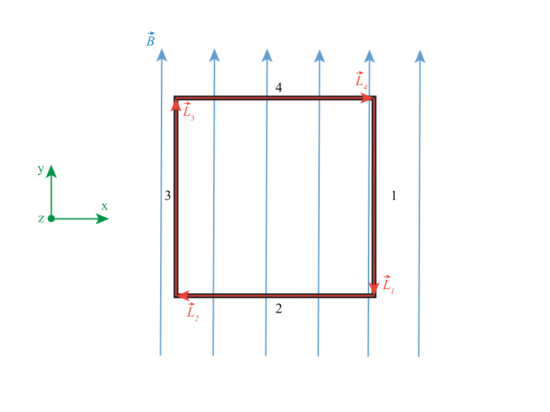
Figure 1: The coordinate system is chosen such that the loop is on the XY plane and the magnetic field points in the positive Y direction. The sub-divisions of the different sides of the loop are also labeled.
We will denote the current flowing through the wire by \(I\), and the length of one side of the square loop by \(L\). We will divide the loop into straight segments which are the sides of the square, denoted by the numbers 1-4 (see the figure above). We can then use the expression for the Lorentz force felt by each segment, namely,
\begin{equation}
\label{lorentza}
\vec{F}=\int_L I\, d\vec{l}\times \vec{B},
\end{equation}
where the integral is taken over the longitude of a segment of the wire (over just one side). Because the current \(I\), the magnetic field \(\vec{B}\) and the direction between each part of the loop and \(\vec{B}\) are constant, we can then take out some factors outside the integral:
\begin{equation}
\label{lorentz}
\vec{F}=\int_L I\, d\vec{l}\times \vec{B}=I \left( \int_L d\vec{l}\right) \times \vec{B}
\end{equation}
And so this is just an integral over a line segment, which gives us a vector whose magnitude is the total length of the segment:
\begin{equation}
\label{lorentz2}
\vec{F}=I\vec{L}\times\vec{B}.
\end{equation}
Here \(\vec{L}\) is a vector whose magnitude is \(L\) (the side of the wire), and its direction is the same as the direction of the current for that segment. Let’s then use this equation to calculate the force over each segment, using a sub-index to differentiate the different segments. But first, notice that in all cases the magnetic field is
\begin{equation}
\label{bfield}
\vec{B}=B\,\hat{\textbf{j}},
\end{equation}
where \(B\) is the magnitude of the magnetic field and \(\hat{\textbf{j}}\) is the unitary vector along the Y direction. Consider now the first segment:
\begin{equation}
\label{lor1}
\vec{F}_1=I\vec{L}_1\times\vec{B}.
\end{equation}
Here the vector \(\vec{L}_1\) can be written as
\begin{equation}
\label{l1}
\vec{L}_1=-L\,\hat{\textbf{j}}
\end{equation}
because the direction of the current in segment 1 goes along the negative Y direction. Using the expressions of equations \eqref{bfield} and \eqref{l1} into \eqref{lor1}, we obtain
\begin{equation}
\vec{F}_1=I(-L\,\hat{\textbf{j}})\times(B\,\hat{\textbf{j}}),
\end{equation}
\begin{equation}
\vec{F}_1=-ILB\,\hat{\textbf{j}}\times\hat{\textbf{j}}
\end{equation}
\begin{equation}
\label{f1}
\vec{F}_1=\vec{0},
\end{equation}
where we have used in the last line the fact that the cross product of two parallel (or anti-parallel) vectors is zero.
Use again equation \eqref{lorentz2} for segment 2, to get
\begin{equation}
\label{lor2}
\vec{F}_2=I\vec{L}_2\times\vec{B}.
\end{equation}
The vector \(\vec{L}_2\) can then be written as
\begin{equation}
\label{l2}
\vec{L}_2=-L\,\hat{\textbf{i}}
\end{equation}
because the direction of the current in segment 2 is in the negative X direction. Using the expressions of equations \eqref{bfield} and \eqref{l2} into \eqref{lor2}, we obtain
\begin{equation}
\vec{F}_2=I(-L\,\hat{\textbf{i}})\times(B\,\hat{\textbf{j}}),
\end{equation}
\begin{equation}
\vec{F}_2=-ILB\,\hat{\textbf{i}}\times\hat{\textbf{j}}
\end{equation}
\begin{equation}
\vec{F}_2=-ILB\,\hat{\textbf{k}},
\end{equation}
where in the last line we used that \(\hat{\textbf{i}}\times\hat{\textbf{j}}=\hat{\textbf{k}}\) (we illustrate this using the right-hand rule below).
 Numerically, we obtain
\begin{equation}
\label{f2}
\vec{F}_2=-(4.3\,\text{A})(0.65\,\text{m})(3.5\,\text{T})\,\hat{\textbf{k}}\approx -9.78\,\text{N}\,\hat{\textbf{k}}.
\end{equation}
Following the reasoning with segment 3, we can write an equivalent expression using equation \eqref{lorentz2}, namely,
\begin{equation}
\label{lor3}
\vec{F}_3=I\vec{L}_3\times\vec{B}.
\end{equation}
The vector \(\vec{L}_3\) is
\begin{equation}
\label{l3}
\vec{L}_3=L\,\hat{\textbf{j}}
\end{equation}
because the direction of the current in segment 3 is in the positive Y direction. Using the expressions of equations \eqref{bfield} and \eqref{l3} into equation \eqref{lor3}, we end up with
\begin{equation}
\vec{F}_3=I(L\,\hat{\textbf{j}})\times(B\,\hat{\textbf{j}}),
\end{equation}
\begin{equation}
\vec{F}_3=ILB\,\hat{\textbf{j}}\times\hat{\textbf{j}}
\end{equation}
\begin{equation}
\label{f3}
\vec{F}_3=\vec{0},
\end{equation}
where we have used in the last line the known result \(\hat{\textbf{j}}\times\hat{\textbf{j}}=\vec{0}\).
Finally we can do the same analysis for segment 4. In that case, we get
\begin{equation}
\label{lor4}
\vec{F}_4=I\vec{L}_4\times\vec{B},
\end{equation}
where the vector \(\vec{L}_4\) is
\begin{equation}
\label{l4}
\vec{L}_4=L\,\hat{\textbf{i}}.
\end{equation}
The direction of the current in segment 4 goes along the positive X direction. Using the expressions of equations \eqref{bfield} and \eqref{l4} into \eqref{lor4}, we obtain
\begin{equation}
\vec{F}_4=I(L\,\hat{\textbf{i}})\times(B\,\hat{\textbf{j}}),
\end{equation}
\begin{equation}
\vec{F}_4=ILB\,\hat{\textbf{i}}\times\hat{\textbf{j}}
\end{equation}
\begin{equation}
\vec{F}_4=ILB\,\hat{\textbf{k}},
\end{equation}
where in the last line we have used again the known result that \(\hat{\textbf{i}}\times\hat{\textbf{j}}=\hat{\textbf{k}}\).
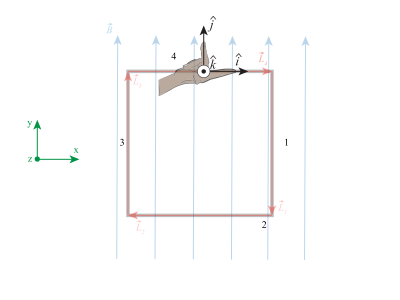
Figure 3: Illustration of the right-hand rule to find the direction of the force exerted on wire 4 of the loop. In this segment, the current moves along the X axis, and so the force points along the positive Z axis. In particular, the final direction is given by \(\hat{\textbf{i}}\times\hat{\textbf{j}}=\hat{\textbf{k}}\)
Numerically, we obtain
\begin{equation}
\label{f4}
\vec{F}_4=(4.3\,\text{A})(0.65\,\text{m})(3.5\,\text{T})\,\hat{\textbf{k}}\approx9.78\,\text{N}\,\hat{\textbf{k}}.
\end{equation}
b) Let us now find the net force and torque that the magnetic field exerts on the square loop. The net force will be the sum of all the forces for all the segments, that is,
\begin{equation}
\label{netforce}
\vec{F}_{\text{net}}=\vec{F}_1+\vec{F}_2+\vec{F}_3+\vec{F}_4.
\end{equation}
Using the results of equations \eqref{f1}, \eqref{f2}, \eqref{f3} and \eqref{f4}, we get
\begin{equation}
\vec{F}_{\text{net}}=-9.78\,\text{N}\,\hat{\textbf{k}}+9.78\,\text{N}\,\hat{\textbf{k}}=\vec{0}.
\end{equation}
To find the torque \(\vec{\tau}\), we must first calculate the magnetic moment of the wire loop \(\vec{\mu}\), whose definition is
\begin{equation}
\label{momamg}
\vec{\mu}=IA\,\hat{\textbf{n}},
\end{equation}
where \(I\) is the current passing through the loop, \(A\) is the area enclosed by the loop and \(\hat{\textbf{n}}\) is a unitary vector which is normal to the area \(A\) and whose direction is given by the right-hand rule. Closing the fingers of the right hand in the direction of the current, the thumb points towards the screen (inside), and so \(\hat{\textbf{n}}\) is \(-\hat{\textbf{k}}\). This is illustrated in figure 4.

Figure 4: We use the right-hand rule to find the direction of the normal vector for the area of the circle. Notice that if we arrange the fingers of the right hand in the direction of the current (which goes clockwise), then the thumb points towards the inside of the screen.
The area enclosed by the loop is the area of a square, that is, \(A=L^2\). Using this in equation \eqref{momamg}, we can then write
\begin{equation}
\label{momag2}
\vec{\mu}=-IL^2\,\hat{\textbf{k}}.
\end{equation}
The expression for the torque in terms of the magnetic moment and the magnetic field is
\begin{equation}
\vec{\tau}=\vec{\mu}\times\vec{B}.
\end{equation}
Use now the expressions in equations \eqref{bfield} and \eqref{momag2}, to write
\begin{equation}
\vec{\tau}=(-IL^2\,\hat{\textbf{k}})\times(B\,\hat{\textbf{j}}),
\end{equation}
\begin{equation}
\vec{\tau}=-IL^2B\,\hat{\textbf{k}}\times \hat{\textbf{j}},
\end{equation}
\begin{equation}
\vec{\tau}=IL^2B\,\hat{\textbf{i}},
\end{equation}
where in the last line we used the fact that \(\hat{\textbf{k}}\times\hat{\textbf{j}}=-\hat{\textbf{i}}\). This is illustrated in figure 5 with the right-hand rule, again:
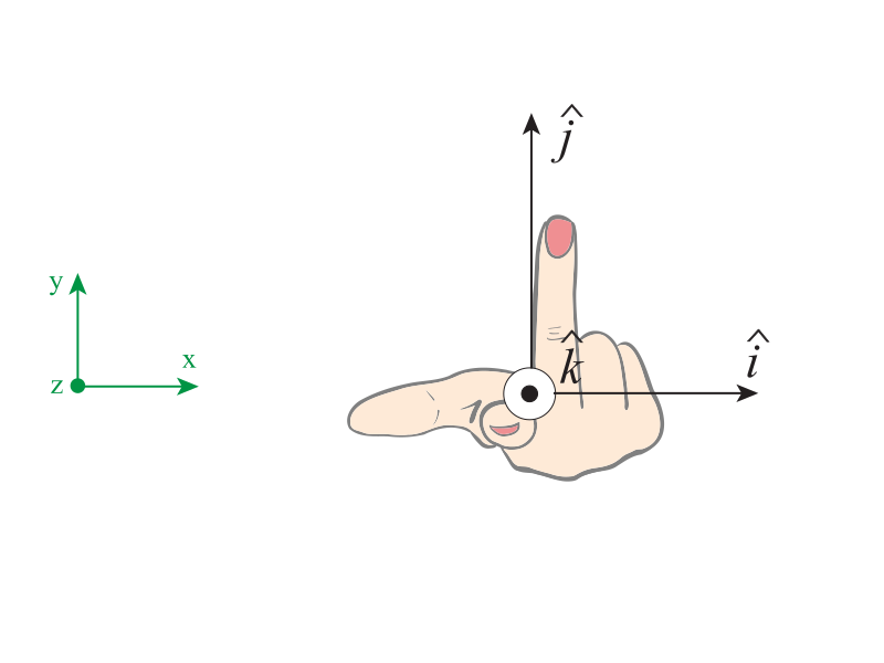
Figure 5: We use the right-hand rule to find the direction of the vector given by \(\hat{\textbf{k}}\times\hat{\textbf{j}}\). Notice that the thumb points in the direction of the negative X axis, and so the result is \(-\hat{\textbf{i}}\).

Leave A Comment