
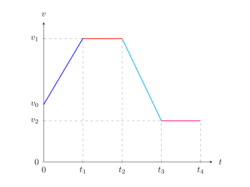
A space capsule re-enters Earth’s atmosphere, and its motion is plotted according to the speed-time graph shown above. Describe the rocket’s motion based on the prompts below.
a) Briefly describe the physical situation on each segment of the plot.
b) Sketch the acceleration vs time plot.
c) Sketch the position vs time plot.
d) In terms of the variables shown in the first figure, calculate the total displacement of the capsule.
(a) First, think about the acceleration as the slope for each segment of the figure, and then use this to try to describe with words what happens in each segment.
(b) Find the slope for each segment.
(c) Find the area under the curve for each segment.
(d) Sum the results obtained in the previous numeral.
(a) From time \(0\) to time \(t_1\) there is a positive acceleration motion. The space capsule is accelerating due to gravity.
From time \(t_1\) to \(t_2\) the acceleration is zero. The space capsule is reaching its terminal velocity (the weight is equal and opposite to the drag force due to the atmosphere).
From time \(t_2\) to \(t_3\), the acceleration is negative. The capsule opens the parachute, thus decreases its velocity.
From time \(t_3\) to \(t_4\) the acceleration is zero. This will be the case of equilibrium when the weight and the drag force exerted by the parachute balance out.
(b) We must first find the acceleration for all time intervals. Since we are dealing with constant acceleration motion, we will use in each interval the equation that defines the acceleration for the constant case, namely:
\begin{equation*}
\vec{a}=\frac{\vec{v}_f-\vec{v}_i}{t_f-t_i}.
\end{equation*}
We can then sketch the graph for acceleration vs time, as seen in the following figure:

Acceleration of the space capsule as it enters the earth as a function of time.
(c) In order to sketch the position graph we must find the displacement \(\Delta x\) through all four regions. We can do this by finding the area underneath the curve of velocity for each region, or by simply using the expression for the position in terms of constant acceleration. We will use the second method, which gives us:
\begin{equation*}
\Delta \vec{x}=\vec{v}_i(t_f-t_i)\,\hat{\textbf{i}}+\frac{1}{2}\vec{a}(t_f-t_i)^2,
\end{equation*}
where \(t_f\) and \(t_i\) are the times at the beginning and end of each region, \(\vec{v}_i\) is the velocity at time \(t_i\) and \(\vec{a}\) is the acceleration in the region. Then, the result is shown in the following figure:

Position of the space capsule as it enters the earth as a function of time.
(d) The total displacement for the capsule will be the sum of the displacements for each segment, explicitly
\begin{equation*}
\Delta \vec{x}_{\text{total}}=\Delta \vec{x}_1+\Delta \vec{x}_2+\Delta \vec{x}_3+\Delta \vec{x}_4,
\end{equation*}
that is,
\begin{equation*}
\Delta \vec{x}_{\text{total}}=\frac{1}{2}(v_1+v_0)t_1\,\hat{\textbf{i}}+v_1(t_2-t_1)\,\hat{\textbf{i}}+\frac{1}{2}(v_2+v_1)(t_3-t_2)\,\hat{\textbf{i}}+v_2(t_4-t_3)\,\hat{\textbf{i}}.
\end{equation*}
For a more detailed explanation of any of these steps, click on “Detailed Solution”.
a) To do a physical analysis of the space capsule entering the Earth, we’ll consider that the positive axis is downwards. Thus, positive velocity and accelerations are considered to be in the direction of gravity’s force, towards the center of the Earth.
From time \(0\) to time \(t_1\) we can see in the graph that, as time increases, so does the velocity. This means that we have a positive acceleration motion. This acceleration is constant because the slope of the curve is constant (it is a straight line). We can imagine that for this time interval, the space capsule is accelerating due to gravity.
From time \(t_1\) to \(t_2\) the speed of the capsule is constant, meaning the acceleration is zero. Physically, this could indicate the moment when the space capsule is reaching its terminal velocity, at which the weight is equal and opposite to the drag force due to the atmosphere (these forces cancel out and then the acceleration becomes zero).
From time \(t_2\) to \(t_3\), the velocity decreases at a constant rate, that is, linearly. This means that the acceleration is negative. Physically, this corresponds to the region when the capsule opens the parachute, thus decreasing the velocity.
From time \(t_3\) to \(t_4\) the velocity is constant meaning there is no acceleration. Physically, this will be the case of equilibrium when the weight and the drag force exerted by the parachute balance out.
b) To sketch the acceleration vs time plot, we must first find the acceleration for all time intervals. Since we are dealing with constant acceleration motion, we will use in each interval the equation that defines the acceleration for the constant case, namely:
\begin{equation}
\label{acel}
\vec{a}=\frac{\vec{v}_f-\vec{v}_i}{t_f-t_i},
\end{equation}
where \(\vec{v}_f\) and \(\vec{v}_i\) are the velocities at times \(t_f\) and \(t_i\) respectively.
For the first region, between 0 and \(t_1\) the velocities are of magnitude \(v_0\) and \(v_1\), and both positive. Hence, we can use equation \eqref{acel} to write an expression for the acceleration in this time interval, namely
\begin{equation}
\vec{a}_1=\frac{v_1\,\hat{\textbf{i}}-v_0\,\hat{\textbf{i}}}{t_1-0},
\end{equation}
which is simplified to
\begin{equation}
\label{}
\vec{a}_1=\frac{v_1-v_0}{t_1}\,\hat{\textbf{i}}.
\end{equation}
Notice that since \(v_1>v_0\), the acceleration \is positive (notice also that we used the unitary vectors to indicate the direction of the velocities).
For the second region, between \(t_1\) and \(t_2\), the velocities are \(v_1\) and again \(v_1\) (and positive). Hence, we can use equation \eqref{acel} to write an expression for the acceleration in this time interval, namely
\begin{equation}
\vec{a}_2=\frac{v_1\,\hat{\textbf{i}}-v_1\,\hat{\textbf{i}}}{t_2-t_1},
\end{equation}
that is,
\begin{equation}
\vec{a}_2=0\,\hat{\textbf{i}},
\end{equation}
which is the result we expected since the velocity does not change.
For the third region, between \(t_2\) and \(t_3\) the velocities are of magnitude \(v_1\) and \(v_2\) (and both are positive). Hence, we can use equation \eqref{acel} to write an expression for the acceleration in this time interval, namely
\begin{equation}
\vec{a}_3=\frac{v_2\,\hat{\textbf{i}}-v_1\,\hat{\textbf{i}}}{t_3-t_2}.
\end{equation}
Notice that since \(v_2<v_1\), the acceleration is negative!
Finally, for the fourth region, between \(t_3\) and \(t_4\) the speeds are \(v_2\) and \(v_2\) (the same speed). Hence, we can use equation \eqref{acel} to write an expression for the acceleration in this time interval, namely
\begin{equation}
\vec{a}_4=\frac{v_2\,\hat{\textbf{i}}-v_2\,\hat{\textbf{i}}}{t_4-t_3},
\end{equation}
which can be simplified to
\begin{equation}
\vec{a}_4=0\,\hat{\textbf{i}},
\end{equation}
a result we expected since the velocity does not change in this region.
We can then sketch the graph for acceleration vs time, as seen in figure 1.
Figure 1: Acceleration of the space capsule as it enters the earth as a function of time.
c) In order to sketch the position graph we must find the displacement \(\Delta x\) through all four regions. We can do this by finding the area underneath the curve of velocity for each region, or by simply using the expression for the position in terms of constant acceleration. We will use the second method, which gives us:
\begin{equation}
\label{deltax}
\Delta \vec{x}=\vec{v}_i(t_f-t_i)\,\hat{\textbf{i}}+\frac{1}{2}\vec{a}(t_f-t_i)^2,
\end{equation}
where \(t_f\) and \(t_i\) are the times at the beginning and end of each region, \(\vec{v}_i\) is the velocity at time \(t_i\) and \(\vec{a}\) is the acceleration in the region. We can use the explicit expression for \(\vec{a}\) given by equation \eqref{acel} into equation \eqref{deltax}, to get
\begin{equation}
\Delta \vec{x}=v_i(t_f-t_i)\,\hat{\textbf{i}}+\frac{1}{2}\left(\frac{v_f-v_i}{t_f-t_i}\right)(t_f-t_i)^2\,\hat{\textbf{i}},
\end{equation}
which simplifies to
\begin{equation}
\Delta \vec{x}=v_i(t_f-t_i)\,\hat{\textbf{i}}+\frac{1}{2}(v_f-v_i)(t_f-t_i)\,\hat{\textbf{i}},
\end{equation}
and after making the sum, this simplifies further to
\begin{equation}
\label{deltax2}
\Delta \vec{x}=\frac{1}{2}(v_f+v_i)(t_f-t_i)\,\hat{\textbf{i}}.
\end{equation}
Using equation \eqref{deltax2} for the first region between 0 and \(t_1\), we find the displacement in this region to be:
\begin{equation}
\Delta \vec{x}_1=\frac{1}{2}(v_1+v_0)(t_1-0)\,\hat{\textbf{i}},
\end{equation}
which simplifies to
\begin{equation}
\label{dx1}
\Delta \vec{x}_1=\frac{1}{2}(v_1+v_0)t_1\,\hat{\textbf{i}}.
\end{equation}
Now, for region 2 we have, using the equation for the displacement given in \eqref{deltax2}, that
\begin{equation}
\Delta \vec{x}_2=\frac{1}{2}(v_1+v_1)(t_2-t_1)\,\hat{\textbf{i}},
\end{equation}
which simplifies to
\begin{equation}
\label{dx2}
\Delta \vec{x}_2=v_1(t_2-t_1)\,\hat{\textbf{i}}.
\end{equation}
For region 3 we obtain, using the equation for the displacement given in \eqref{deltax2}, that
\begin{equation}
\label{dx3}
\Delta \vec{x}_3=\frac{1}{2}(v_2+v_1)(t_3-t_2)\,\hat{\textbf{i}}.
\end{equation}
Finally, for region 4, we use equation \eqref{deltax2} to get the displacement:
\begin{equation}
\label{dx4}
\Delta \vec{x}_4=\frac{1}{2}(v_2+v_2)(t_4-t_3)\,\hat{\textbf{i}},
\end{equation}
which simplifies to
\begin{equation}
\Delta \vec{x}_4=v_2(t_4-t_3)\,\hat{\textbf{i}}.
\end{equation}
Figure 2: Position of the space capsule as it enters the earth as a function of time.
To sketch the graph, we know that in the region of positive acceleration (region 1) and positive velocity, the position must increase as a parabola opening upwards. In the regions where the acceleration is zero (regions 2 and 4) and the velocity is positive, the position must increase linearly. In the region where the acceleration is negative (region 3) and velocity is positive, the position must increase as a parabola opening downwards. Taking all of this into account and supposing that the initial position is \(x_0\), we have the graph, as shown in the next figure. The starting point is \(x_0\). At time \(t_1\) the position is \(\vec{x}_0+\Delta \vec{x}_1\), at time \(t_2\) the position is \(\vec{x}_0+\Delta \vec{x}_1+\Delta \vec{x}_2\), at time \(t_3\) the position is \(\vec{x}_0+\Delta \vec{x}_1+\Delta \vec{x}_2+\Delta \vec{x}_3\) and the position at time \(t_4\) is \(\vec{x}_0+\Delta \vec{x}_1+\Delta \vec{x}_2+\Delta \vec{x}_3+\Delta \vec{x}_4\).
d) The total displacement for the capsule will be the sum of the displacements given by equations \eqref{dx1}, \eqref{dx2}, \eqref{dx3} and \eqref{dx4}, explicitly
\begin{equation}
\Delta \vec{x}_{\text{total}}=\Delta \vec{x}_1+\Delta \vec{x}_2+\Delta \vec{x}_3+\Delta \vec{x}_4,
\end{equation}
that is,
\begin{equation}
\Delta \vec{x}_{\text{total}}=\frac{1}{2}(v_1+v_0)t_1\,\hat{\textbf{i}}+v_1(t_2-t_1)\,\hat{\textbf{i}}+\frac{1}{2}(v_2+v_1)(t_3-t_2)\,\hat{\textbf{i}}+v_2(t_4-t_3)\,\hat{\textbf{i}}.
\end{equation}


Leave A Comment