A Circuit and a Mass!

a) Use Ohm’s Law to solve for the current. The direction of the current can be determined by the position of the battery.

b) Use Ampere’s Law to solve for the magnetic field induced by the cable and find the magnetic force. Then, use Newton’s Second Law to determine the mass.

a) Using Ohm’s Law and solving for \(I\), we get:

\begin{equation*}
I=\frac{V}{R},
\end{equation*}

which, numerically, is

\begin{equation*}
I\approx 16.7\,\text{A}.
\end{equation*}

b) Ampere’s Law states:

\begin{equation*}
\oint \vec{B} \cdot d \vec{r} = \mu_0 I_c.
\end{equation*}

The right side of the equation becomes \(B 2 \pi r\). The enclosed current is \(I\). Then, solving for \(B\) we get:

\begin{equation*}
B = \frac{\mu_0 I}{2 \pi r}.
\end{equation*}

The magnetic force is:

\begin{equation*}
{F}= \frac{\mu_0 I I’}{2\pi x}.
\end{equation*}

Using Newton’s Second Law on the wire, we get:

\begin{equation*}
F – mg = 0,
\end{equation*}

where, replacing the recently found magnetic force, and solving for \(m\), we get:

\begin{equation*}
m=\frac{L\mu_0 I I’}{2\pi x g}.
\end{equation*}

Plugging in numerical values yields:

\begin{equation*}
m \approx 0.6 \, \text{g}.
\end{equation*}

For a more detailed explanation of any of these steps, click on “Detailed Solution”.

a) For the first part we are asked to find the direction of the current in the circuit and its value between points \(a\) and \(b\). Let’s start by using Ohm’s law to find the magnitude of the current \(I\), namely

\begin{equation}
\label{ohm}
V=IR,
\end{equation}

where \(V\) is the voltage in the battery and \(R\) the value of the resistance. Solving for \(I\) in equation \eqref{ohm}, we get

\begin{equation}
I=\frac{V}{R},
\end{equation}

which numerically is

\begin{equation}
I=\frac{200\,\text{V}}{12\,\Omega},
\end{equation}

\begin{equation}
I\approx 16.7\,\text{A}.
\end{equation}

The direction of the current is shown in figure 1, where the current flows from the positive terminal of the battery to the negative terminal. Thus it goes from \(b\) to \(a\).

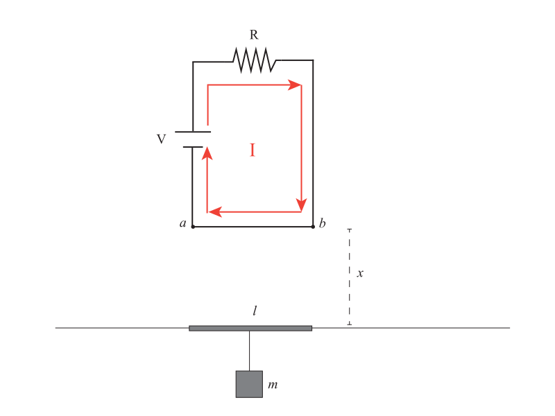
Figure 1: Direction of the current \(I\) through the circuit. The segment \(a-b\) is separated a distance \(x\) from the wire of length \(l\) and mass \(m\).

b) Let’s consider now a 20 A current flowing in the light wire and an unknown mass \(m\) hanging from it. We first need to calculate the direction in which the current must flow for the mass to remain in balance. Because the length of both wires (the segment \(a-b\) and the light wire) is much greater than the distance that separates them, we can consider them as being infinite and parallel for the purposes of calculation. The next step is to find the magnetic force that an infinite wire produces at some distance \(r\) over another wire. One can find this force in two sub-steps: (i) we first find the magnetic field produced by a wire at some distance \(r\), and (ii) we then use Lorentz force to find the force felt by a different wire due to the magnetic field found in (i) (if the reader already knows the force that a wire feels due to a different wire, then the reader can skip the next couple of paragraphs, but here we want to derive the result from some basic principles).

Finding the magnetic field produced by a wire:

Let’s then first consider a long, straight wire carrying a current \(i\). First, we will use the fact that the magnetic field lines always go in circles around a straight wire, and the direction can be obtained from the right-hand rule. In particular, point the thumb of your right hand in the direction of the current, and then wrap the wire with the other fingers. The way in which your fingers are wrapped determines the direction of the field around the wire, as in figure 2.

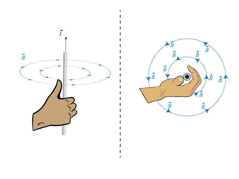
Figure 2: On the left: Magnetic field lines \(\vec{B}\) produced by a wire with current \(\vec{I}\). Notice that we use the right-hand rule to find the direction of the magnetic field.  If you place the thumb of your right hand in the direction of the current and wrap the wire with the other fingers, then the direction in which the other fingers point indicates whether the magnetic field is clockwise or counterclockwise. On the right: A view from above, with the current flowing out of the screen. Notice that the magnetic field is counter-clockwise

Notice from figure 2 that each circle of radius \(r\) has magnetic field lines of constant magnitude, always pointing in the tangential direction (always pointing counter-clockwise). If do the same reasoning but for the problem at hand, we will get the following (see figure 3).

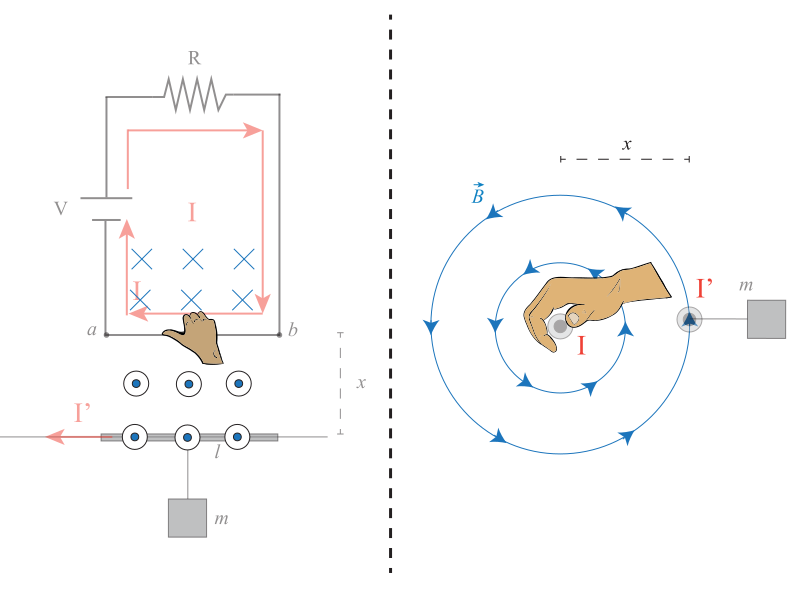
Figure 3: On the left: Direction of the magnetic field \(\vec{B}\) generated by the current flowing through the segment \(a-b\). We find the direction using the right-hand rule, where the thumb points in the direction of the current and the other fingers indicate the direction of the field (counter-clockwise or clockwise around the wire). The dots indicate the magnetic field coming out of the screen while the crosses represent the magnetic field entering the screen. On the right: Use the right-hand rule to find the direction of circulation of the magnetic field. The current \(I’\) passing through the light wire \(I’\) is also shown.

Now, the right-hand rule gave us the direction, but to find the magnitude of the field produced by the wire, we will use Ampère’s Law, which states that

\begin{equation}
\label{eqref:ampere1}
\oint \vec{B} \cdot d \vec{r} = \mu_0 I_c.
\end{equation}

This integral is a path integral along with a closed path P (that we are free to choose) that encloses a current \(I_c\). Here, \(d \vec{r}\) is a differential length element that points along the path of integration,  and \(\mu_0\) is the permeability constant (also known as the ‘magnetic constant’).  Hence, we can use this equation to find the magnetic field produced by the \(a-b\) segment with current \(I\).

In this case, we can easily perform the integration because of the symmetry of the magnetic field, which always goes in circles, as explained before. In order to perform the integration, we first need to choose a path. Clearly, we want a path such that \(\vec{B} \cdot d \vec{r}\) (the term to be integrated) is as simple as possible.  So in our case, we choose the path of integration to be a circle of radius \(r\) around the cable. As we can see in figure 4, this path is convenient because the field \(\vec{B}\) and the path differential \(d \vec{r}\) are always parallel to one another:

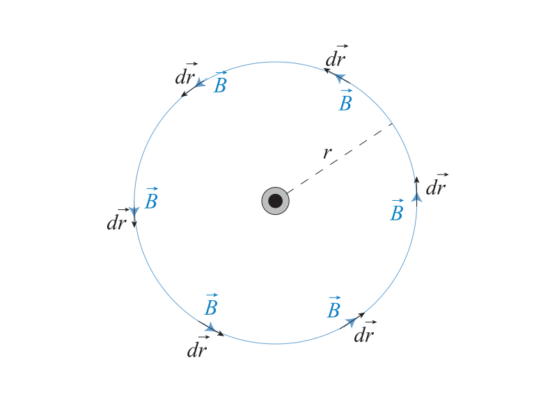
Figure 4: To apply Ampère’s Law, we choose as a path a circle that encloses the cable (the current) at its middle point. Notice that this path guarantees that the magnetic field vector is always (at any point on the circle) parallel to the line differential \(d \vec{r}\) (since they are parallel, and since the magnetic field has the same magnitude all around the circle, then the product \(\vec{B} \cdot d \vec{r} = B dr\) is a constant that can be written as \(Bdr\)).

Thus, Ampère’s Law becomes

\begin{equation}
\label{eqref:ampere2}
\oint \vec{B} \cdot d \vec{r} = \oint B dr = B \oint dr = \mu_0 I,
\end{equation}

where we used the fact that \(I_c = I\), given that the current enclosed by this circle is \(I\), and where we also took \(B\) out of the integration because it is constant at any point around the circle. Finally, all we need to compute is \(\oint dr \), which is the path integral of the line differential along the circle. In other words, this integration corresponds the total length of the path in question which is just the perimeter of the circle. Hence

\begin{equation}
\label{eqref:ampere2b}
B \oint dr = 2 \pi r = \mu_0 I
\end{equation}

Thus,

\begin{equation}
\label{eqref:ampere 3}
B 2 \pi r = \mu_0 I,
\end{equation}

and solving for B, we get

\begin{equation}
\label{wirefield}
B = \frac{\mu_0 I}{2 \pi r}.
\end{equation}

We have then found the magnitude of the wire’s magnetic field at a distance \(r\) (and we already found the direction).

Magnetic Force Felt by a Wire

We move on to sub-step two, where we will find the magnetic force that the other wire feels due to the magnetic field produced by the first wire, which we just computed. This force is simply given by Lorentz force law in the absence of an electric field, and which states that the force felt by a charge \(q\) moving with velocity \(vec{v}\) in the presence of a magnetic field is

\begin{equation}
\label{florentz}
{\vec{F}}=q\vec{v}\times \vec{B}.
\end{equation}

In the present case, we want to find the force felt by the current \(I’\) on the bottom wire. But recall that current is just charge over time, and so \(I’=q/t\), from which it follows that \(I’t=q\). Use this in the previous equation to get

\begin{equation}
\label{florentz2}
{\vec{F}}=I’t\vec{v}\times \vec{B}.
\end{equation}

And now use that the velocity is the displacement over time, that is,

\begin{equation}
\label{velocity}
\vec{v}=\frac{\vec{L}}{t},
\end{equation}

where \(\vec{L}\) is a vector that points in the direction of the current over the bottom wire, and whose magnitude is \(l\) (the length of the segment). If we use this result in equation \eqref{florentz2}, we get

\begin{equation}
\label{florentz3}
{\vec{F}}=I’t\frac{\vec{L}}{t}\times \vec{B}.
\end{equation}

The time cancels, and we get

\begin{equation}
\label{florentz4}
{\vec{F}}=I'{\vec{L}}\times \vec{B}.
\end{equation}

Now, before we continue, let’s find the magnitude of this force. Using the definition of the magnitude of the cross product, we have

\begin{equation}
\label{florentz5}
{F}=I’LB \sin \theta,
\end{equation}

where \(\theta\) is the angle between the vectors. Notice that \(\vec{L}\) goes either horizontally to the left or to the right (depends on whether the current \(I’\) goes left or right). And as we explained before,  \(\vec{B}\) (the field produced by the top wire) goes outside the screen on the region where the bottom wire is placed. Hence, \(\vec{B}\) and \(\vec{L}\) will always be perpendicular, meaning that the angle between them is \(90^{\circ}\). And so the previous equation becomes

\begin{equation}
\label{florentz6}
{F}=I’LB.
\end{equation}

Before we replace here the magnitude of the magnetic field found with equation \eqref{wirefield}, let’s think about the direction of this force (we already know it must be perpendicular to both \(\vec{L}\) and \(\vec{B}\) because the force comes from the cross product between these vectors, but there are still two open options; either the force goes upwards or downwards, in both cases, it would be perpendicular). We can simply use the right-hand rule to determine the direction:

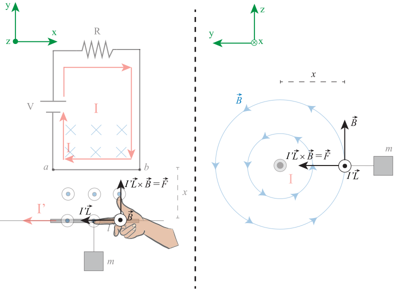
Figure 5: Left: Direction of the force \(\vec{F}\) exerted by the magnetic field generated by the segment \(a-b\) on the light wire. Again, the direction of the force is found using the right-hand rule. Notice that if both currents point in the same direction then the force goes upwards, meaning that the wires get attracted. Right: Transverse view of the two wires and the magnetic field generated by the segment \(a-b\). The force is attractive between both wires.

From the diagram, it is clear that if the currents are parallel, then the bottom wire feels attracted to the top wire, which is what we need if we want the bottom wire to hold the mass in equilibrium. The reader can easily notice that if the currents were anti-parallel, then the wires would repel one another (use again the right-hand rule, but with the opposite direction for the current \(I’\)).

Finally, use the magnetic field found with equation \eqref{wirefield} back in equation \eqref{florentz6} to get

\begin{equation}
\label{fmag}
{F}=I’L\frac{\mu_0 I I’}{2\pi x}=\frac{\mu_0 I I’}{2\pi x}
\end{equation}

The forces exerted on the light wire are then the weight of the mass \(m\) and the force \(F\) (that we drew upwards) required so that the light wire remains in equilibrium. As we explained earlier, we need the currents to be parallel (point in the same direction) so that the force \(F\) is a force of attraction between the light wire and the wire of segment \(a-b\). Making a free-body diagram over the bottom wire, we then obtain what is shown in figure 6.

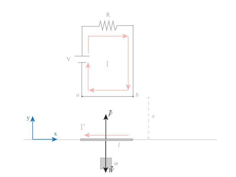
Figure 6: Free-body diagram of the light wire with the magnetic force \(\vec{F}\) upwards and the weight \(\vec{W}=-mg\,\hat{\textbf{j}}\) downwards. Notice the coordinate system used.

We can now write Newton’s second law:

\begin{equation}
\label{newton2}
\sum \vec{F}=m\vec{a}.
\end{equation}

But in equilibrium, there is no acceleration and so we get

\begin{equation}
\label{newton3}
\sum \vec{F}=\vec{0}.
\end{equation}

In this case \(\sum \vec{F}\) is the weight of the mass \(m\) directed downwards, plus the force \(F\) directed upwards. We ignore the mass of the light wire since we will suppose it is much less than \(m\). From equation \eqref{newton3}, we get

\begin{equation}
-mg\,\hat{\textbf{j}}+F\,\hat{\textbf{j}}=\vec{0}.
\end{equation}

Focusing on just the magnitude, this becomes

\begin{equation}
\label{newton4}
-mg+F=0,
\end{equation}

where \(g\) is the gravitational acceleration of Earth. Solving for \(m\), we get

\begin{equation}
m=\frac{F}{g}.
\end{equation}

Using the expression for \(F\) given in equation \eqref{fmag}, we finally get

\begin{equation}
m=\frac{L\mu_0 I I’}{2\pi x g}.
\end{equation}

Using the numerical values in the SI units, so that \(L=0.3\,\text{m}\) and \(x=3.4\times10^{-3}\,\text{m}\), we get

\begin{equation}
m=\frac{(0.3\,\text{m})(4\pi\times 10^{-7}\,\text{T m A}^{-1})(16.7\,\text{A})(20\,\text{A})}{2\pi (3.4\times 10^{-3}\,\text{m})(9.81\,\text{m/s}^2)},
\end{equation}

\begin{equation}
m\approx 6\times 10^{-4}\,\text{kg}=0.6\,\text{g}.
\end{equation}

You need to be registered and logged in to take this quiz. Log in or Register