

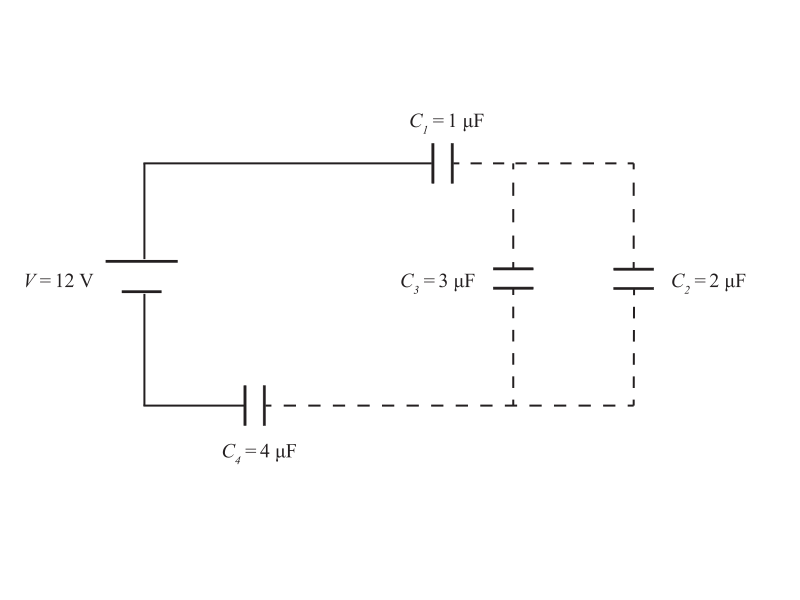
For the circuit in the figure, find:
(a) The equivalent capacitance.
(b) The charge stored in capacitor 3.
(a) In order to find the equivalent capacitance of the circuit, we need to identify groups of capacitors that are in series (which all have the same charge) or in parallel (which will have the same voltage), and apply the equations for the equivalent capacitance accordingly. We need to repeat this procedure until we reduce the circuit to a single (equivalent) capacitor. Once we have the equivalent capacitance of the circuit, we can use the definition of capacitance, and the layout of the different sets of capacitors (i.e. whether they are connected in series of in parallel) to find their charges and voltages. We can do this sequentially as we expand the circuit back from a single equivalent capacitor into the circuit shown in the first figure.
As shown in the next figure, capacitors \(C_2\) and \(C_3\) share the same continuous wire connection at both of their ends. Assuming that the wires have negligible resistance, this implies that \(C_2\) and \(C_3\) are subjected to the same voltage and thus are connected in parallel. For capacitors connected in parallel, the equivalent capacitance is simple the sum of the capacitances of each capacitor. Therefore, their equivalent capacitance \(C’_1\) is given by
\begin{equation}
\label{EQ:CP1}
C’_1 = C_2 + C_3.
\end{equation}
After replacing \(C_2\) and \(C_3\) by their equivalent capacitor the circuit becomes as shown in the next figure.

Now, notice that \(C_1, C’_1\), and \(C_4\) are connected contiguously and the wiring between them does not branch. Hence, they are connected in series. For a group of capacitors connected in series, the inverse of the equivalent capacitance equals the sum of the inverse of the capacitances of these capacitors. Therefore, the equivalent resistance \(C’_2\) of capacitors \(C_1, C’_1\), and \(C_4\) is given by
\begin{equation}
\frac{1}{C’_2} = \frac{1}{C_1} + \frac{1}{C’_1} + \frac{1}{C_4},
\end{equation}
and inverting the fractions gives
\begin{equation}
C’_2 = \frac{1}{ \frac{1}{C_1} + \frac{1}{C’_1} + \frac{1}{C_4}}.
\end{equation}
After substituting equation \eqref{EQ:CP1} into this equation we obtain
\begin{equation}
\label{EQ:CP2}
C’_2 = \frac{1}{ \frac{1}{C_1} + \frac{1}{C_2 + C_3 } + \frac{1}{C_4} }.
\end{equation}
Now, if we replace \(C_1, C’_1\) and \(C_4\) with their equivalent capacitor, we obtain the circuit shown in the next figure.

We have reduced the circuit to a single resistor connected to the source. Therefore, \(C’_2\) is the equivalent capacitance \(C_{\text{eq}}\) of the circuit, meaning:
\begin{equation}
C_{\text{eq}} = C’_2,
\end{equation}
and from equation \eqref{EQ:CP2} we obtain:
\begin{equation}
C_{\text{eq}} = \frac{1}{ \frac{1}{C_1} + \frac{1}{ C_2 + C_3 } + \frac{1}{C_4} }.
\end{equation}
Finally, plugging in numerical values gives us:
\begin{equation}
\label{EQ:CEQ}
C_{\text{eq}} = \frac{1}{\frac{1}{1 \ \mu\text{F}} + \frac{1}{2 \ \mu\text{F}+ 3 \ \mu\text{F}} + \frac{1}{4 \ \mu\text{F}} } = \frac{20}{29} \ \mu\text{F} = 0.69 \ \mu\text{F}.
\end{equation}
(b) Now, we need to find the charged stored in Capacitor 3. Let us recall that the capacitance \(C\) of a capacitor is defined as the charge \(Q\) stored in it divided by the potential difference \(V\) at which it is subjected i.e.
\begin{equation}
\label{EQ:C}
C = \frac{Q}{V}.
\end{equation}
We can rewrite this expression as:
\begin{equation}
\label{EQ:Q}
Q = CV,
\end{equation}
and
\begin{equation}
\label{EQ:V}
V = \frac{Q}{C},
\end{equation}
in order to find either the charge \(Q\) or the voltage \(V\) in terms of the other two variables.
We can now use equations \eqref{EQ:Q} and \eqref{EQ:V} to find the charges and voltages of all capacitors as we expand the circuit from the one with a single equivalent capacitance in the fourth figure until we obtain the charge of capacitor 3.
In the reduced circuit of the fourth figure, the potential difference at which capacitor \(C’_2\) is subjected is the same as the voltage of the source. This is because \(C’_2\) is connected to the source from both ends without any other component in between. Therefore, using eq. \eqref{EQ:Q} we can write the charge \(Q’_2\) of this capacitor as
\begin{equation}
\label{EQ:QP2}
Q’_2 = C’_2 V,
\end{equation}
where \(C’_2\) is given by eq. EQ:CP2 and \(V = 12\) V is the voltage of the source. Since these two variables are known, the value of \(Q’_2\) is known.
Recall that \(C’_2\) is the equivalent capacitance of capacitors \(C_1, C’_1\), and \(C_4\), which are connected in series according to the third figure. Therefore, their have the same stored charge. In particular for \(C’_1\) we can write
\begin{equation}
Q’_1 = Q’_2,
\end{equation}
and substituting eq. \eqref{EQ:QP2} gives
\begin{equation}
\label{EQ:QP1}
Q’_1 = C’_2 V.
\end{equation}
Since we now know the charge and capacitance of this capacitor, we can use eq. \eqref{EQ:V} to find its voltage. The voltage \(V’_1\) of capacitor \(C’_1\) is given by
\begin{equation}
V’_1 = \frac{Q’_1}{C’_1},
\end{equation}
and substituting eq. \eqref{EQ:QP1} yields
\begin{equation}
\label{EQ:VP1}
V’_1 = \frac{C’_2 V}{ C’_1}.
\end{equation}
Now, \(C’_1\) is the equivalent capacitance of capacitors \(C_2\) and \(C_3\), which are connected in parallel according to the second figure. Therefore, they are subjected to the same voltage. In particular, the voltage \(V_3\) of capacitor \(C_3\) is given by
\begin{equation}
V_3 = V’_1,
\end{equation}
and substituting eq. \eqref{EQ:VP1} gives
\begin{equation}
\label{EQ:V3}
V_3 = \frac{C’_2 V}{ C’_1}.
\end{equation}
Finally, from equation \eqref{EQ:Q}, the charge of capacitor 3 is thus given by
\begin{equation}
Q_3 = C_3 V_3,
\end{equation}
and substituting eq. \eqref{EQ:V3} yields
\begin{equation}
Q_3 = C_3 \frac{C’_2 V}{ C’_1} = C_3 V \frac{C’_2}{C’_1},
\end{equation}
where \(C’_2\) is given by eq. \eqref{EQ:CP2} and \(C’_1\) is given by eq. \eqref{EQ:CP1}. If we insert these equations we obtain
\begin{equation}
Q_3 = C_3 V \frac{ \frac{1}{ \frac{1}{C_1} + \frac{1}{ C_2 + C_3 } + \frac{1}{C_4} }}{C_2 + C_3 }.
\end{equation}
Finally, substituting numerical values gives
\begin{equation}
Q_3 = (3\ \mu \text{F}) (12 \ \text{V}) \frac{\frac{1}{ \frac{1}{ 1\ \mu \text{F} } + \frac{1}{2\ \mu \text{F} + 3\ \mu \text{F} } + \frac{1}{4\ \mu \text{F}} } } { 2\ \mu \text{F} + 3\ \mu \text{F} }
= \frac{144}{29} \ \mu \text{C} = 4.966\ \mu \text{C}.
\end{equation}

Leave A Comment