Non-Uniform Charge Distribution on a Circle Section!

Use the definition of a differential electric field. Write the differential charge in terms of the linear density, and write the distance in terms of the angle. Use these formulae to integrate among the given angles.

The differential electric field is:

\begin{equation*}
d\vec{E}=\frac{dq}{4\pi\epsilon_0 r^2}\,\hat{\textbf{r}},
\end{equation*}

where \( \hat{\textbf{r}} = – \sin \theta \, \hat{\textbf{i}} – \cos \theta \hat{\textbf{j}}\). The charge is \(dq = \lambda ds\) and \(ds = a d \theta\). Then, integrating at both sides, the electric field can be written as:

\begin{equation*}
\vec{E}=\int_{-\frac{\pi}{4}}^{\frac{\pi}{4}} \frac{\sec \theta \,d\theta}{4\pi \epsilon_0 a}(-\sin(\theta)\,\hat{\textbf{i}}-\cos(\theta)\,\hat{\textbf{j}}),
\end{equation*}

where the density \(\lambda = \sec \theta\) was already substituted.

By performing the integration, the \(\hat{\textbf{i}}\) component is zero. This gives us:

\begin{equation*}
\vec{E}=-\frac{1}{8\epsilon_0 a}\,\hat{\textbf{j}}.
\end{equation*}

For a more detailed explanation of any of these steps, click on “Detailed Solution”.

To calculate the electric field \(\vec{E}\) produced by the charge distribution, we’ll partition the circle’s relevant section into very small segments of charge \(dq\) and length \(ds\) (see Figure 1 below). Then, we can consider these small segments as point charges that produce a small electric field \(d\vec{E}\) given by the following equation:

\begin{equation}
d\vec{E}=\frac{dq}{4\pi\epsilon_0 r^2}\,\hat{\textbf{r}},
\end{equation}

where \(r\) is the distance from charge \(dq\) to the point where the electric field is being calculated (P) and \(\hat{\textbf{r}}\) is the unitary vector in the direction of the vector that goes from charge \(dq\) to point P. Since we want the electric field for the whole segment, we need to add all the contributions of all charges \(dq\). After doing so, we end up with the integral equation

\begin{equation}
\label{efield1}
\int d\vec{E}=\int \frac{dq}{4\pi\epsilon_0 r^2}\,\hat{\textbf{r}}.
\end{equation}

The left-hand side of equation \eqref{efield1} is the electric field \(\vec{E}\). So,

\begin{equation}
\label{efield2}
\vec{E}=\int \frac{dq}{4\pi\epsilon_0 r^2}\,\hat{\textbf{r}}.
\end{equation}

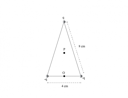
Now, in order to continue and be able to use this equation, we need to express the unitary vector \(\hat{\textbf{r}}\) in terms of other variables given by the geometry of the problem. First, we’ll draw vector \(\vec{r}\)  as is seen in figure 1.

Figure 1: We place the coordinate system at the center of the circumference. The electric field \(\vec{dE}\) generated by the charge differential \(dq\) of length \(ds\) is shown along with the distance vector \(\vec{r}\). The field is written in terms of its X and Y’s components according to angle \(\theta\).

In general, for all charges \(dq\), the vector \(\vec{r}\) has a magnitude \(r\) equal to the radius of the semicircle \(a\)

\begin{equation}
\label{ere}
r=a,
\end{equation}

and the direction will be given in terms of the angle \(\theta\), measured from the vertical as seen in figure 1. So, we can write

\begin{equation}
\label{vecere}
\vec{r}=-a\sin(\theta)\,\hat{\textbf{i}}-a\cos(\theta)\,\hat{\textbf{j}}.
\end{equation}

The unitary vector \(\hat{\textbf{r}}\) can be calculated as the ratio of \(\vec{r}\) and \(r\). Explicitly,

\begin{equation}
\label{runit}
\hat{\textbf{r}}=\frac{\vec{r}}{r}.
\end{equation}

Using the results of equations \eqref{ere} and \eqref{vecere} into equation \eqref{runit}, we have

\begin{equation}
\hat{\textbf{r}}=\frac{-a\sin(\theta)\,\hat{\textbf{i}}-a\cos(\theta)\,\hat{\textbf{j}}}{a},
\end{equation}

which becomes

\begin{equation}
\label{runit2}
\hat{\textbf{r}}=-\sin(\theta)\,\hat{\textbf{i}}-\cos(\theta)\,\hat{\textbf{j}}.
\end{equation}

Using the result of equations \eqref{ere} and \eqref{runit2} into equation \eqref{efield2}, we obtain

\begin{equation}
\label{efield3}
\vec{E}=\int\frac{dq}{4\pi \epsilon_0 a^2}(-\sin(\theta)\,\hat{\textbf{i}}-\cos(\theta)\,\hat{\textbf{j}}).
\end{equation}

We are given the charge density distribution \(\lambda\), which in terms of \(dq\) and \(ds\) can be written as

\begin{equation}
\lambda=\frac{dq}{ds},
\end{equation}

which can be solved for \(dq\) to get

\begin{equation}
\label{dq}
dq=\lambda\, ds.
\end{equation}

Because \(ds\) is a differential arc length, it relates to the radius and a differential arc angle \(d\theta\) as follows

\begin{equation}
\label{ds}
ds=a\,d\theta.
\end{equation}

Using the result of equation \eqref{ds} into equation \eqref{dq}, we finally obtain an expression for \(dq\) in terms of geometric variables that we can use to integrate; namely,

\begin{equation}
\label{dq2}
dq=\lambda a\,d\theta.
\end{equation}

Then we can replace \(dq\) in equation \eqref{efield3} using the expression of equation \eqref{dq2} to get

\begin{equation}
\label{efield4}
\vec{E}=\int_{\theta_1}^{\theta_2}\frac{\lambda a\,d\theta}{4\pi \epsilon_0 a^2}(-\sin(\theta)\,\hat{\textbf{i}}-\cos(\theta)\,\hat{\textbf{j}}),
\end{equation}

where the limits of the integral are given in terms of the angles \(\theta_1\) and \(\theta_2\). Taking out the constant terms in equation \eqref{efield4} and using the expression for the charge density \(\lambda=\sec(\theta)\), we obtain

\begin{equation}
\label{efield5}
\vec{E}=\frac{a}{4\pi\epsilon_0 a^2}\int_{\theta_1}^{\theta_2}d\theta\sec(\theta)(-\sin(\theta)\,\hat{\textbf{i}}-\cos(\theta)\,\hat{\textbf{j}}).
\end{equation}

Using the trigonometric identity \(\sec(\theta)=\frac{1}{\cos(\theta)}\), we can write equation \eqref{efield5} as

\begin{equation}
\label{efield6}
\vec{E}=\frac{1}{4\pi\epsilon_0 a}\int_{\theta_1}^{\theta_2}\frac{d\theta}{\cos(\theta)}(-\sin(\theta)\,\hat{\textbf{i}}-\cos(\theta)\,\hat{\textbf{j}}),
\end{equation}

where we have also cancelled the \(a\) in the numerator with an \(a\) in the denominator outside the integral.

Using the distributive law in equation \eqref{efield6}, we finally get

\begin{equation}
\label{efield7}
\vec{E}=\frac{1}{4\pi\epsilon_0 a}\int_{\theta_1}^{\theta_2} d\theta\left(-\frac{\sin(\theta)}{\cos(\theta)}\,\hat{\textbf{i}}-\frac{\cos(\theta)}{\cos(\theta)}\,\hat{\textbf{j}}\right),
\end{equation}

which, after simplification, becomes

\begin{equation}
\label{efield8}
\vec{E}=\frac{1}{4\pi\epsilon_0 a}\int_{\theta_1}^{\theta_2} d\theta\left(-\tan(\theta)\,\hat{\textbf{i}}-1\,\hat{\textbf{j}}\right).
\end{equation}

From the figure above, we can also see that the limits are \(\theta_1=-\pi/4\) and \(\theta_2=\pi/4\), so we must solve the integral

\begin{equation}
\label{efield9}
\vec{E}=\frac{1}{4\pi\epsilon_0 a}\int_{-\frac{\pi}{4}}^{\frac{\pi}{4}} d\theta\left(-\tan(\theta)\,\hat{\textbf{i}}-1\,\hat{\textbf{j}}\right).
\end{equation}

Which can be divided as follows

\begin{equation}
\label{efield10}
\vec{E}=-\frac{1}{4\pi\epsilon_0 a}\left(\int_{-\frac{\pi}{4}}^{\frac{\pi}{4}} d\theta\tan(\theta)\,\hat{\textbf{i}}+\int_{-\frac{\pi}{4}}^{\frac{\pi}{4}} d\theta \,\hat{\textbf{j}}\right).
\end{equation}

Performing the integrals we get

\begin{equation}
\vec{E}=-\frac{1}{4\pi\epsilon_0 a}\left(\ln|\sec(\theta)|\,\hat{\textbf{i}}+\theta\,\hat{\textbf{j}}\right)\Big|_{-\frac{\pi}{4}}^{\frac{\pi}{4}},
\end{equation}

which after evaluating is

\begin{equation}
\vec{E}=-\frac{1}{4\pi \epsilon_0 a}\left((\ln|\sec(\pi/4)|-\ln|\sec(-\pi/4)|)\,\hat{\textbf{i}}+\left(\frac{\pi}{4}-\left(-\frac{\pi}{4}\right)\right)\,\hat{\textbf{j}}\right).
\end{equation}

The component alongside the X axis cancels out, and then we get

\begin{equation}
\vec{E}=-\frac{1}{4\pi\epsilon_0 a}\left(0\,\hat{\textbf{i}}+\frac{\pi}{2}\,\hat{\textbf{j}}\right).
\end{equation}

The final expression for the electric field will be then

\begin{equation}
\vec{E}=-\frac{1}{8\epsilon_0 a}\,\hat{\textbf{j}}.
\end{equation}

You need to be registered and logged in to take this quiz. Log in or Register